Read PtyRAD Output hdf5

• Created with PtyRAD 0.1.0b13

• Requires PtyRAD >= 0.1.0b13

• Documentation: https://ptyrad.readthedocs.io/en/latest/

• PtyRAD paper: https://doi.org/10.1093/mam/ozaf070

• PtyRAD arXiv: https://arxiv.org/abs/2505.07814

• Zenodo record: https://doi.org/10.5281/zenodo.15273176

• Box folder: https://cornell.box.com/s/n5balzf88jixescp9l15ojx7di4xn1uo

• Youtube channel: https://www.youtube.com/@ptyrad_official

Before running this notebook, you must first follow the instruction in README.md to:

1. Create the Python environment with all dependant Python packages like PyTorch

2. Activate that python environment

3. Install ptyrad package into your activated Python environement (only need to install once)

Note: This notebook is designed to demonstrate how to load the PtyRAD reconstructed model output from hdf5 files

Author: Chia-Hao Lee, cl2696@cornell.edu

00. Setup working directory and imports

import os
import numpy as np
import matplotlib.pyplot as plt

# Set this to your desired working directory so you can easily access the data, model, param files
work_dir = "H:/workspace/ptyrad/"

os.chdir(work_dir)
print("Current working dir: ", os.getcwd())
# Note that the output/ directory will be automatically generated under your working directory

Current working dir:  H:\workspace\ptyrad

from ptyrad.io.load import load_ptyrad
from ptyrad.plotting import plot_scan_positions, plot_probe_modes, plot_loss_curves, plot_slice_thickness

01. Setup file path and load the output hdf5

model_path   = "output/tBL_WSe2/20250908_full_N16384_dp128_flipT100_random32_p6_1obj_1slice_plr1e-4_oalr5e-4_oplr5e-4_slr2e-3_orblur0.4_ozblur1.0_mamp0.03_4.0_oathr0.96_oposc_sng1.0_spr0.1/model_iter0200.hdf5"

# PtyRAD model output is just normal hdf5 file so you can open it just like normal hdf5
# But it's strongly recommended to use `load_ptyrad` to handle different data types, strings encoding, dicts, lists, and their nested structures for convenience 

ckpt         = load_ptyrad(model_path) # The loaded checkpoint (ckpt) is just a nested python dict

02. Basic structure of the model output

print("ckpt: ")
for k in ckpt.keys():
    print('  ', k)

ckpt: 
   avg_iter_t
   avg_losses
   batch_losses
   dz_iters
   indices
   iter_times
   loss_iters
   model_attributes
   niter
   optim_state_dict
   optimizable_tensors
   output_path
   params
   ptyrad_version
   random_seed

• model_attributes contains important metadata for the ptychography forward model (i.e., propagator, dx, dk, crop positions, etc.)

• optimizable_tensors stores the AD-optimized tensors for object, probe, position, tilts, and thickness

• params keeps a copy of the loaded PtyRAD param

print(f'model_attributes: \n  {ckpt["model_attributes"].keys()}\n')
print(f'optimizable_tensors: \n  {ckpt["optimizable_tensors"].keys()}\n')
print(f'params: \n  {ckpt["params"].keys()}\n')

model_attributes: 
  dict_keys(['H', 'N_scan_fast', 'N_scan_slow', 'crop_pos', 'detector_blur_std', 'dk', 'dx', 'lr_params', 'obj_preblur_std', 'omode_occu', 'probe_int_sum', 'scan_affine', 'shift_probes', 'slice_thickness', 'start_iter', 'tilt_obj'])

optimizable_tensors: 
  dict_keys(['obj_tilts', 'obja', 'objp', 'probe', 'probe_pos_shifts', 'slice_thickness'])

params: 
  dict_keys(['constraint_params', 'hypertune_params', 'init_params', 'loss_params', 'model_params', 'params_path', 'recon_params'])

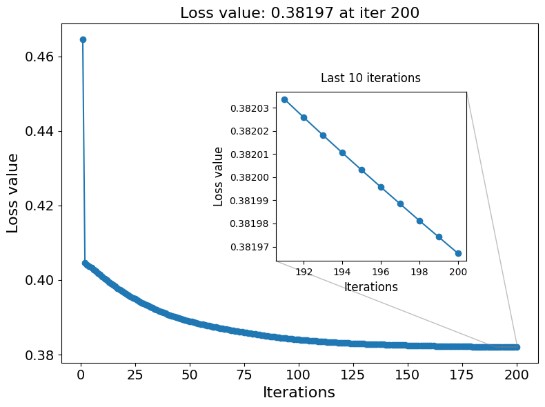
plot_loss_curves(ckpt['loss_iters'])

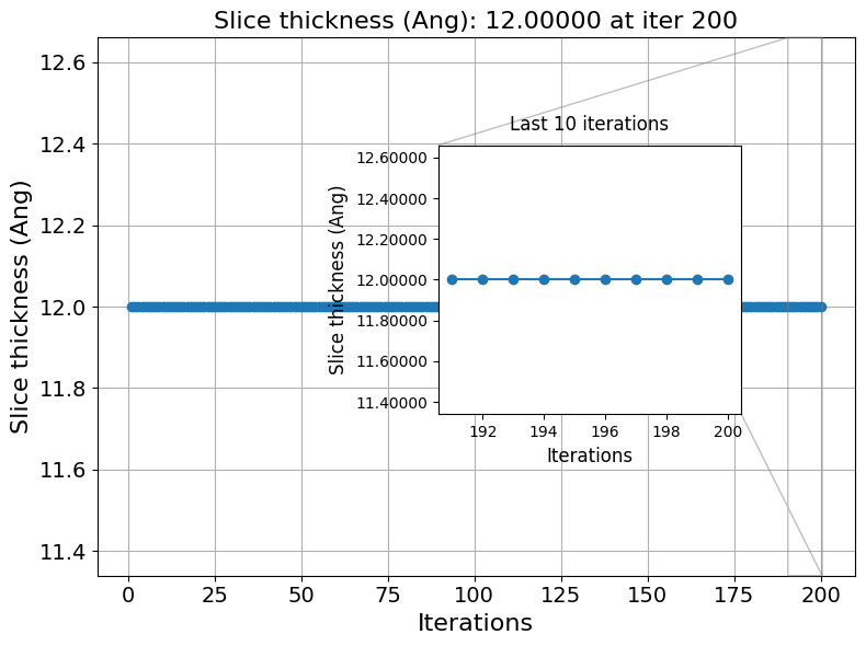
plot_slice_thickness(ckpt['dz_iters'])

03. Retrieve reconstructed obj, probe, positions

03.A Object

obja = ckpt['optimizable_tensors']['obja']
objp = ckpt['optimizable_tensors']['objp']
objc = obja * np.exp(1j*objp) # c for complex
print(objc.shape) # (omode, Nz, Ny, Nx)

(1, 1, 583, 583)

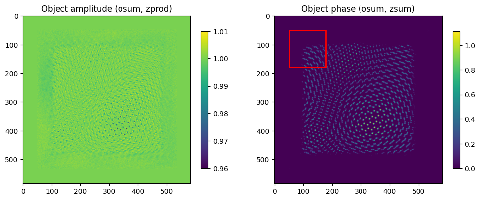
import matplotlib.patches as patches

fig, axs = plt.subplots(nrows=1, ncols=2, figsize=(12,6))
im0 = axs[0].imshow(obja.sum(0).prod(0))
im1 = axs[1].imshow(objp.sum(0).sum(0))
fig.colorbar(im0, shrink=0.6)
fig.colorbar(im1, shrink=0.6)
axs[0].set_title('Object amplitude (osum, zprod)') # amplitude along depth is multiplicative
axs[1].set_title('Object phase (osum, zsum)')

# (x, y) is bottom-left corner in pixel coords, (w, h) is width/height
square = patches.Rectangle((50, 50), 128, 128, linewidth=2,
                           edgecolor='red', facecolor='none')
axs[1].add_patch(square)  # add to right image

plt.show()

# Note that there're blank spaces around the object because we'll need to fit the probe completely inside the object canvas for element-wise multiplication
# The red box denotes the probe window with the probe located in the center, see 03.C Position for more details about relative alignment

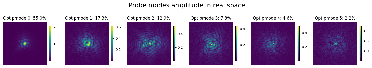
03.B Probe

probe = ckpt['optimizable_tensors']['probe']
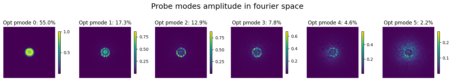
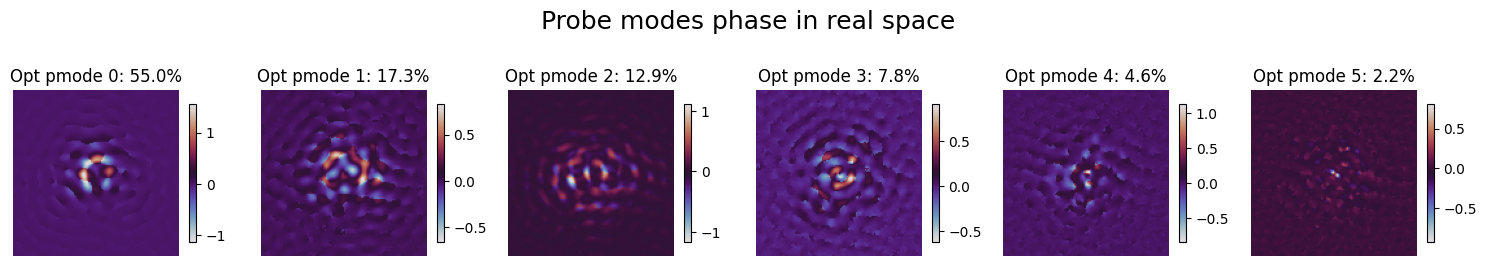
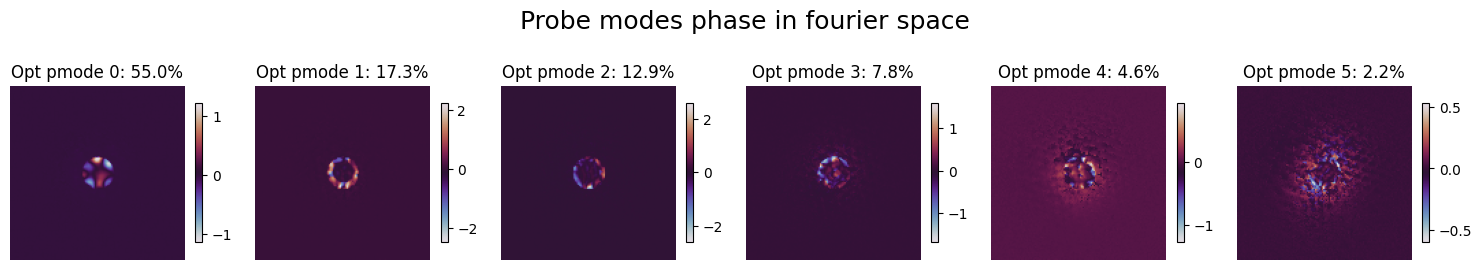
print(probe.shape) # (pmode, Ny, Nx), note that probe is stored as complex-valued probe wavefunction in real space, locating in the window center

(6, 128, 128)

plot_probe_modes(opt_probe=probe, amp_or_phase='amplitude', real_or_fourier='real')
plot_probe_modes(opt_probe=probe, amp_or_phase='amplitude', real_or_fourier='fourier')
plot_probe_modes(opt_probe=probe, amp_or_phase='phase', real_or_fourier='real')
plot_probe_modes(opt_probe=probe, amp_or_phase='phase', real_or_fourier='fourier')

03.C Probe position

crop_pos = ckpt['model_attributes']['crop_pos']
probe_pos_shifts = ckpt['optimizable_tensors']['probe_pos_shifts']
pos = crop_pos + probe_pos_shifts # In unit of real space object px
print(pos.shape)

# Note that crop_pos is a fixed array with integer values. PtyRAD only optimizes sub-px position shifts relative to these initial crop_pos.
# pos is defined at the top-left corner of the probe window, so there's an offset of (Npix/2, Npix/2) between the cropping position, and the actual probe position on object

(16384, 2)

crop_pos

array([[ 49,  49],
       [ 49,  52],
       [ 49,  55],
       ...,
       [407, 401],
       [407, 404],
       [407, 407]], dtype=int32)

probe_pos_shifts

array([[ 0.67257774,  3.2575853 ],
       [ 1.6509179 ,  2.3556314 ],
       [ 3.1341972 ,  3.66328   ],
       ...,
       [-2.4141347 , -3.514011  ],
       [-3.0580354 , -2.7943096 ],
       [-2.6611648 , -3.638554  ]], dtype=float32)

pos

array([[ 49.67257774,  52.25758529],
       [ 50.65091789,  54.35563135],
       [ 52.13419724,  58.66328001],
       ...,
       [404.58586526, 397.48598909],
       [403.94196463, 401.20569038],
       [404.33883524, 403.3614459 ]])

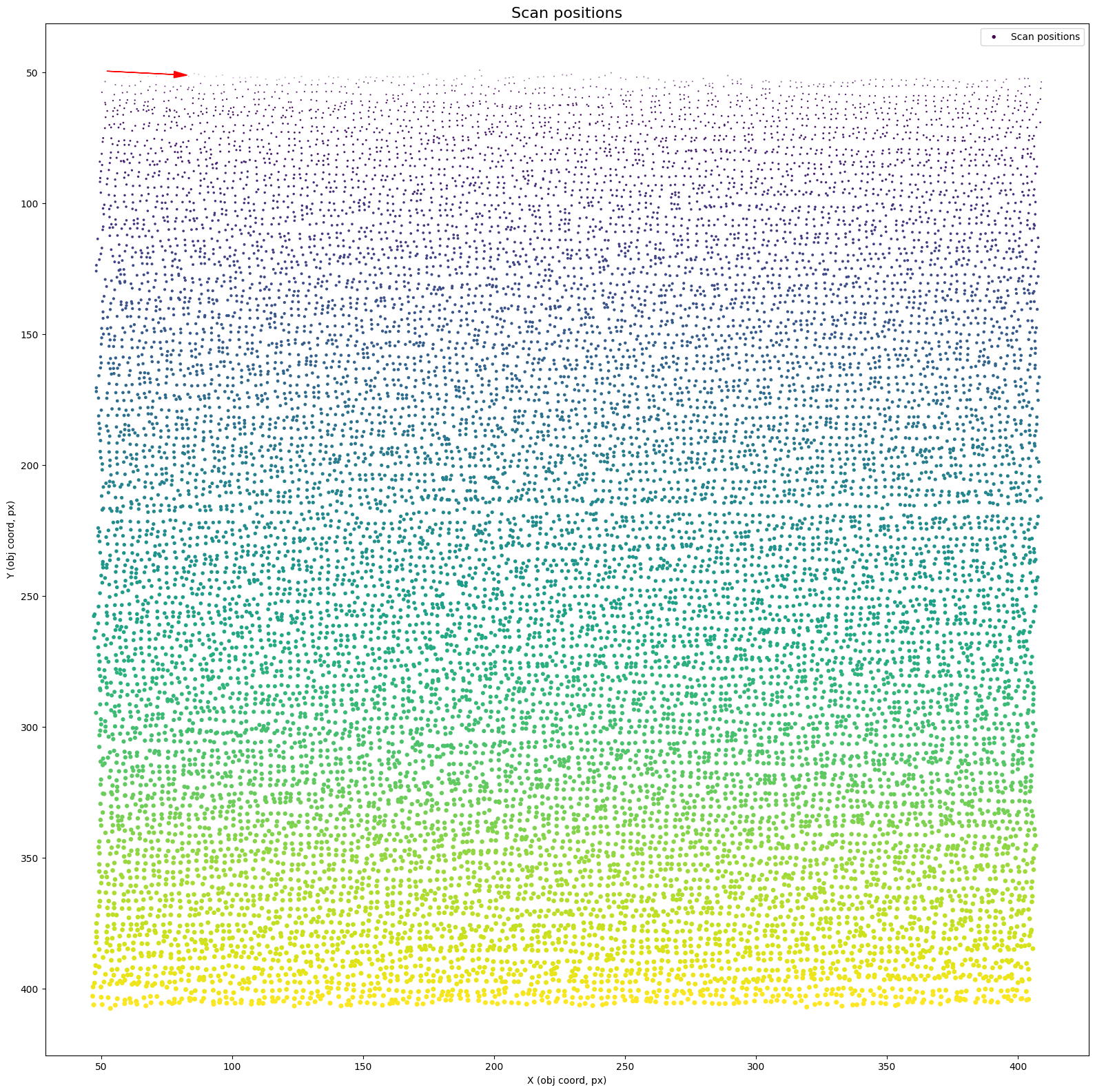
plot_scan_positions(pos)

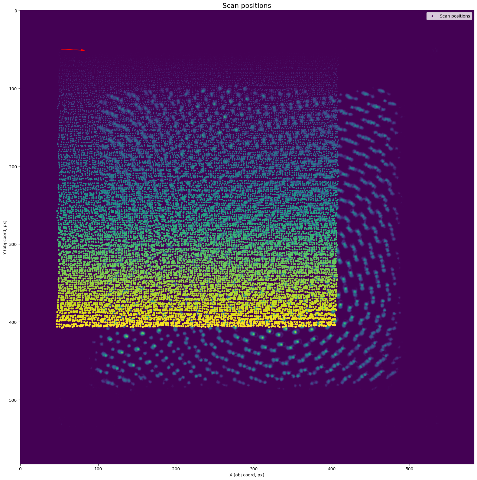
plot_scan_positions(pos, img=objp.sum(0).sum(0), offset=(0,0)) # The scatter points denote the "cropping position", which are the top-left corner of the each probe windows

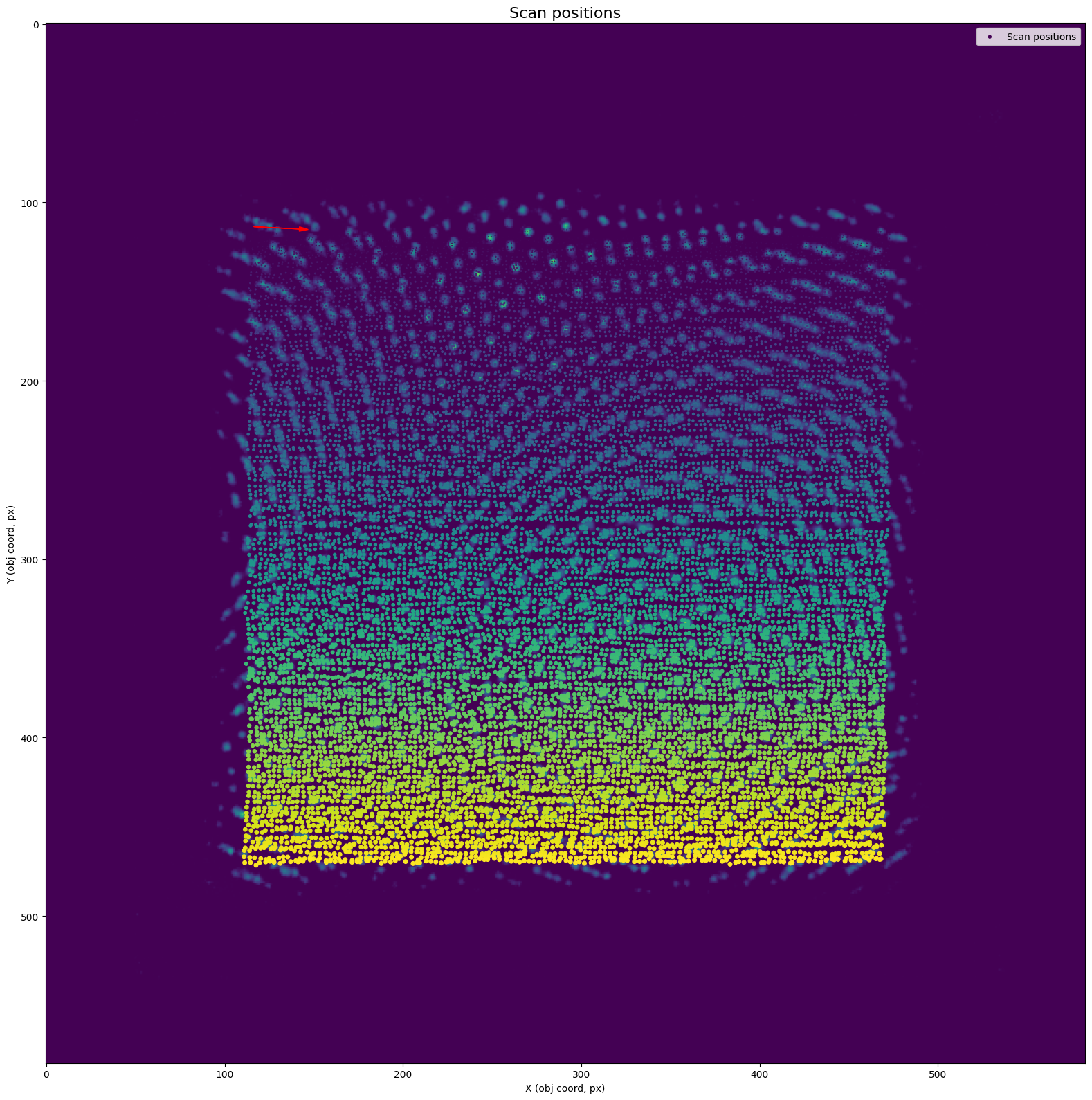
plot_scan_positions(pos, img=objp.sum(0).sum(0), offset=np.array(probe.shape[1:])/2) # The scatter points now denote the actual probe positions on object

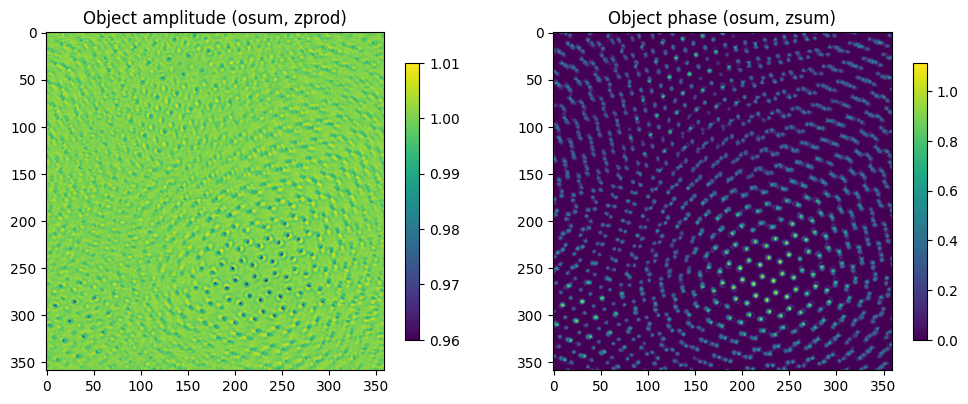
03.D Crop object by the scanning FOV

img_crop_pos = crop_pos + np.array(probe.shape[-2:])//2
y_min, y_max = img_crop_pos[:,0].min(), img_crop_pos[:,0].max()
x_min, x_max = img_crop_pos[:,1].min(), img_crop_pos[:,1].max()

objp_crop = objp[:, :, y_min-1:y_max, x_min-1:x_max]
obja_crop = obja[:, :, y_min-1:y_max, x_min-1:x_max]

fig, axs = plt.subplots(nrows=1, ncols=2, figsize=(12,6))
im0 = axs[0].imshow(obja_crop.sum(0).prod(0))
im1 = axs[1].imshow(objp_crop.sum(0).sum(0))
fig.colorbar(im0, shrink=0.6)
fig.colorbar(im1, shrink=0.6)
axs[0].set_title('Object amplitude (osum, zprod)') # amplitude along depth is multiplicative
axs[1].set_title('Object phase (osum, zsum)')
plt.show()