Get local object tilts#
Created with PtyRAD 0.1.0b13
Requires PtyRAD >= 0.1.0b13
Documentation: https://ptyrad.readthedocs.io/en/latest/
PtyRAD paper: https://doi.org/10.1093/mam/ozaf070
PtyRAD arXiv: https://arxiv.org/abs/2505.07814
Zenodo record: https://doi.org/10.5281/zenodo.15273176
Box folder: https://cornell.box.com/s/n5balzf88jixescp9l15ojx7di4xn1uo
Youtube channel: https://www.youtube.com/@ptyrad_official
Before running this notebook, you must first follow the instruction in README.md to:
Create the Python environment with all dependant Python packages like PyTorch
Activate that python environment
Install
ptyradpackage into your activated Python environement (only need to install once)
Note: This notebook is designed for estimating position-dependent object tilt
Author: Chia-Hao Lee, cl2696@cornell.edu
STO data credit: Dr. Hongbin Yang, hy643@cornell.edu
Notes about object tilt#
Object tilt != beam tilt, because the latter has strong influence to aberrations.
In practice, object tilt is often simulated with a tilted propagator, see Kirkland eqn. 6.99, 2010 edition.
This tilted propagator is equivalent to shifted slices for small angles (i.e., 1-5 deg), see Cowley JM (1975) Diffraction physics, 2nd edn.
Fundamentally, electron waves would be attracted by nuclei even they’re laterally shifted. This gives exactly the channeling effect.
Incorporating object tilt into ptycho reconstruction does NOT really “remove” the tilt, it is more of a tilted view of the reconstructed object by moving tilt from the object to the propagator.
Experimental pattern with obj tilt can be reconstructed either as:
Straight-down propagator + object with shifted slices
Tilted propagator + object with aligned slices
Due to the thick slices (i.e., 1 nm), incorporating tilt into the propagator could potentially reduce the reconstructed atomic column width (simple projection trigonometry)
If you apply position-dependent tilt, it is essentially bending the object grid non-uniformly, so technically the px size becomes position dependent as well.
Depends on the amount of the tilt, this position-dependent-tilt-induced object distortion could be up to a few to 10 pm so treat it carefully if you want to do detailed strcutural analysis
Not much we can do if the obj tilt is changing along the beam propagation direction (i.e, bended specimen)
In practice you can estimate the global object tilt from PACBED or Kikuchi pattern, and often times PtyRAD can handle object tilt just fine by reconstructing into shifted slices.
Although estimating obj tilts from shifted slices is quite accurate, it requires a successful multislice ptycho reconstructions. For a quick alternative, you can run a sliding window PACBED to estimate pos-dependent tilts as well.
For position-dependent tilt, it is strongly recommended to provide initial guess with this notebook or other methods.
00. Setup working directory and imports#
import os
import numpy as np
import matplotlib.pyplot as plt
import matplotlib.gridspec as gridspec
from skimage.feature import blob_log
from scipy.ndimage import center_of_mass
from scipy.interpolate import griddata
from scipy.optimize import curve_fit

from ptyrad.io.load import load_ptyrad
from ptyrad.io.handlers import save_array

# Set this to your desired working directory so you can easily access the data, model, param files
work_dir = "H:/workspace/ptyrad/"

os.chdir(work_dir)
print("Current working dir: ", os.getcwd())
# Note that the output/ directory will be automatically generated under your working directory
Current working dir: H:\workspace\ptyrad
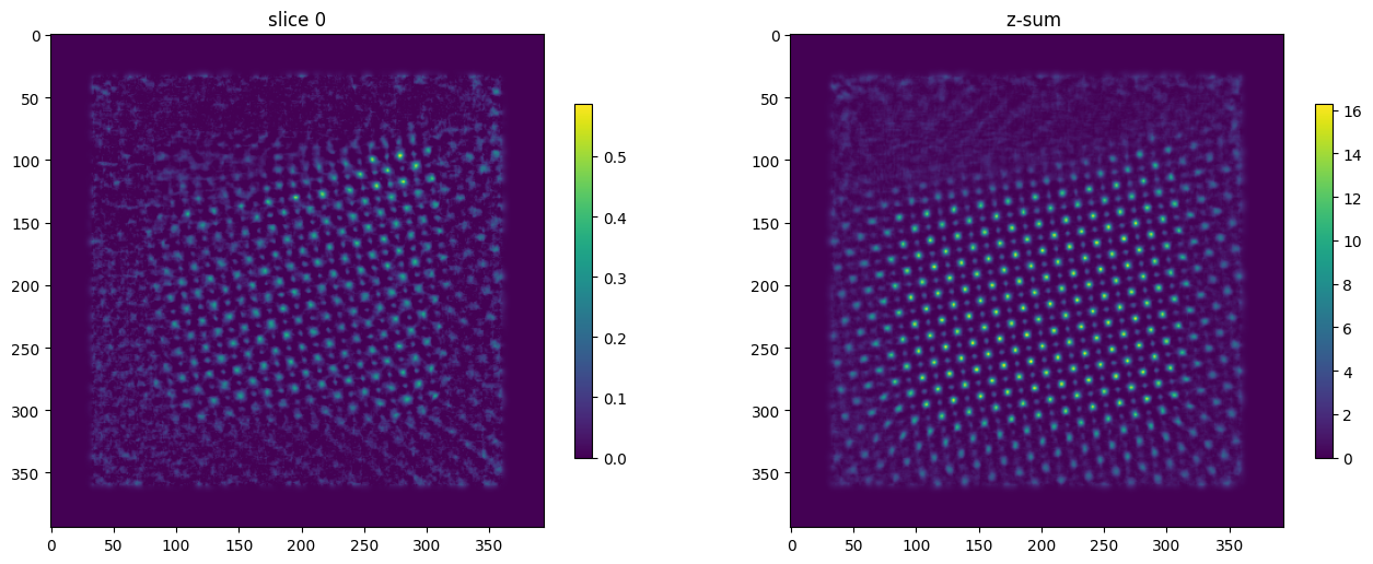
01. Load the 3D image stack#
model_path = "H:/workspace/ptyrad_work/output/Hongbin_STO_16/20250923_full_N4096_dp128_sparse32_p4_1obj_30slice_dz10_plr1e-4_oalr5e-4_oplr5e-4_slr5e-4_dpblur1.0_orblur0.4_ozblur1.0_oathr0.95_oposc_sng1.0_spr0.1/model_iter0200.hdf5"
ckpt = load_ptyrad(model_path)
dx = ckpt['model_attributes']['dx']
slice_thickness = ckpt['optimizable_tensors']['slice_thickness']
imstack = ckpt['optimizable_tensors']['objp'].sum(0) # objp (omode, Nz, Ny, Nx) so we first reduce the omode dimension
Npix = ckpt['optimizable_tensors']['probe'].shape[-1] # Probe window size

# Plot the selected slice and z-sum
idx = 0
fig, axs = plt.subplots(1,2, figsize=(16,6))
im0 = axs[0].imshow(imstack[idx])
im1 = axs[1].imshow(imstack.sum(0))

axs[0].set_title(f"slice {idx}")
axs[1].set_title("z-sum ")

fig.colorbar(im0, shrink=0.7)
fig.colorbar(im1, shrink=0.7)
plt.show()
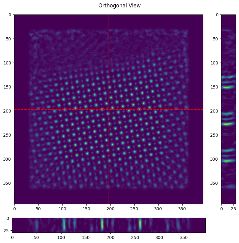
# Plot the orthogonal view, obj tilt is visualized by the slanted atomic column along depth dimension
ortho_view = (imstack.shape[-2]//2, imstack.shape[-1]//2) # y, x in object pixel
fig = plt.figure(figsize=(8,8))
gs = gridspec.GridSpec(2, 2, figure=fig, width_ratios=[1,0.1], height_ratios=[1,0.1])

ax0 = fig.add_subplot(gs[0, 0])
ax1 = fig.add_subplot(gs[0, 1])
ax2 = fig.add_subplot(gs[1, 0])

im0 = ax0.imshow(imstack.sum(0), aspect='equal')
im1 = ax1.imshow(imstack[:, :, ortho_view[1]].T, aspect='equal')
im2 = ax2.imshow(imstack[:, ortho_view[0], :], aspect='equal')

ax0.axhline(ortho_view[0], color='red', linestyle='--')
ax0.axvline(ortho_view[1], color='red', linestyle='--')

plt.suptitle('Orthogonal View')
plt.tight_layout()
plt.show()
02. Extract atom locations from targeted slices#
# Choose the 2 slices from imstack
slice_t = 5
slice_b = 25
height = (slice_b - slice_t)*slice_thickness
print(f"The height difference between slices {(slice_t, slice_b)} is {height:.2f} Ang")
target_stack = imstack[[slice_t,slice_b]]
# Adjust Blob detection parameters accordingly, see: https://scikit-image.org/docs/0.25.x/api/skimage.feature.html#skimage.feature.blob_log
blobs = blob_log(target_stack[0], min_sigma=1, max_sigma=5, overlap=0.1, threshold = 0.20, exclude_border=(Npix//2, Npix//2))
print(f"Found {len(blobs)} blobs with mean radius of {1.414*blobs.mean(0)[-1]:.2f} px or {dx*1.414*blobs.mean(0)[-1]:.2f} Ang")
# Plot the detected blobs
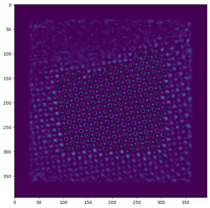
fig, ax = plt.subplots(figsize=(8,8))
ax.imshow(target_stack[0])
for blob in blobs:
y, x, r = blob
c = plt.Circle((x, y), r, linewidth=2, fill=False)
ax.add_patch(c)
plt.show()
The height difference between slices (5, 25) is 200.00 Ang
Found 159 blobs with mean radius of 2.38 px or 0.45 Ang
03. Extend blob detection to all intermediate slices#
window_size = 13 # Ideally the window should contain only 1 lattice point (i.e., 1 atomic column or 1 pair of dumbells)
row_start = np.uint32(blobs[:,0]-window_size//2)
row_end = np.uint32(blobs[:,0]+window_size//2+1)
col_start = np.uint32(blobs[:,1]-window_size//2)
col_end = np.uint32(blobs[:,1]+window_size//2+1)
coord_t = np.zeros((len(blobs),2))
coord_b = np.zeros((len(blobs),2))
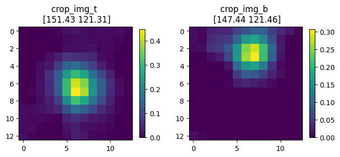
for i in range(len(blobs)):
crop_img_t = target_stack[0][row_start[i]:row_end[i], col_start[i]:col_end[i]]
crop_img_b = target_stack[1][row_start[i]:row_end[i], col_start[i]:col_end[i]]
coord_t[i] = center_of_mass(crop_img_t) + blobs[i,:-1] - window_size//2
coord_b[i] = center_of_mass(crop_img_b) + blobs[i,:-1] - window_size//2
shift_vecs = coord_b - coord_t # This is the needed tilt to correct the obj tilt so it's pointing from top to bottom
# Plot the cropped window for CoM fitting
fig, axs = plt.subplots(1,2, figsize=(8,4))
im0 = axs[0].imshow(crop_img_t)
im1 = axs[1].imshow(crop_img_b)
axs[0].set_title(f"crop_img_t \n {coord_t[-1].round(2)}")
axs[1].set_title(f"crop_img_b \n {coord_b[-1].round(2)}")
fig.colorbar(im0, shrink=0.7)
fig.colorbar(im1, shrink=0.7)
plt.show()
04. Plot the position-dependent tilt vectors#
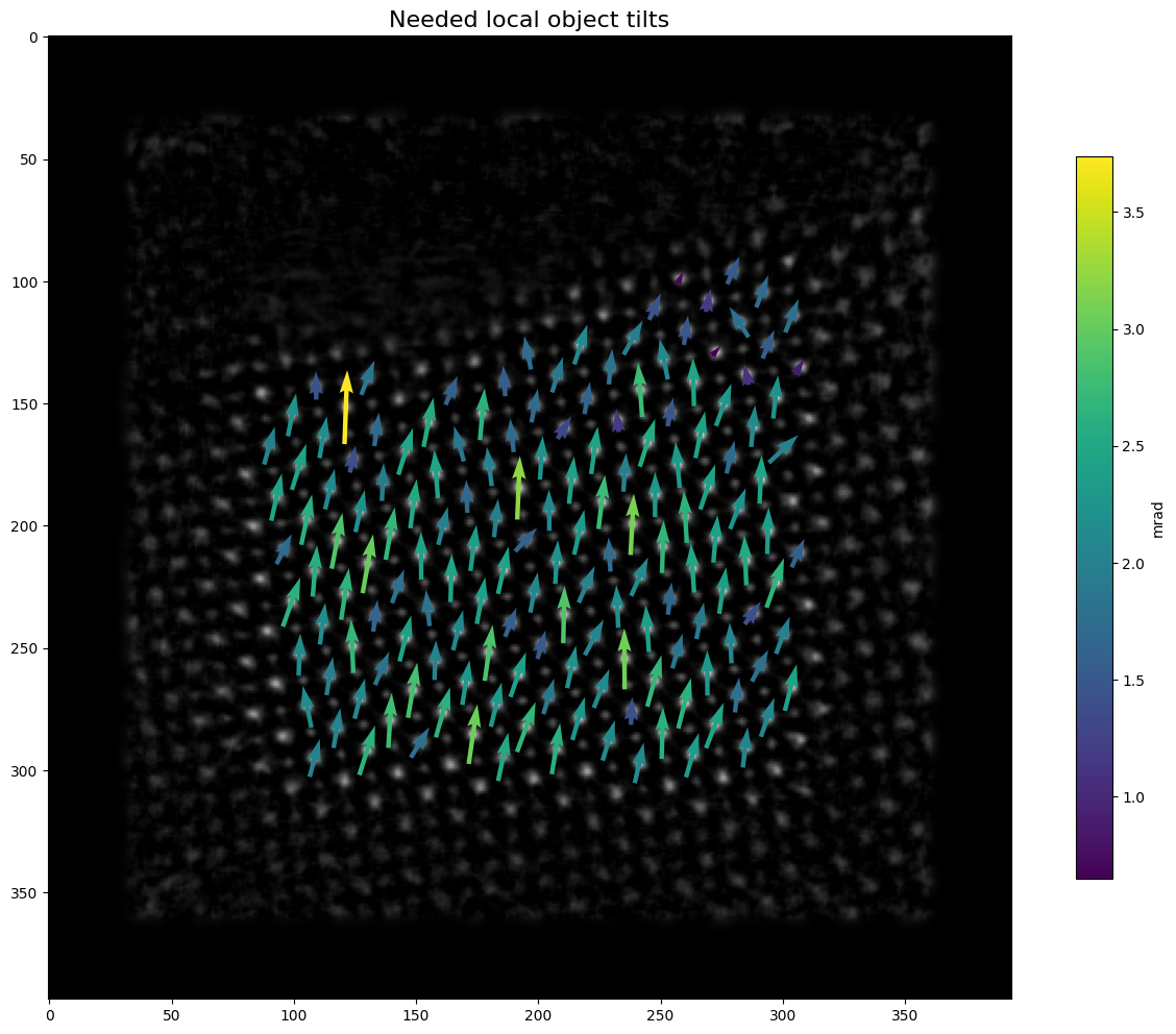
# Plot the tilt vectors
X = coord_t[:,1]
Y = coord_t[:,0]
U = shift_vecs[:,1]
V = shift_vecs[:,0]
M = np.arctan(np.hypot(U,V)*dx/height)*1e3

fig, ax = plt.subplots(figsize=(16,12))
plt.title("Needed local object tilts", fontsize=16)
ax.imshow(target_stack[0], cmap='gray')
q = ax.quiver(X, Y, U, V, M, pivot='mid', angles='xy', scale_units='xy')
cbar = fig.colorbar(q, shrink=0.75)
cbar.ax.set_ylabel('mrad')
plt.show()
05. Interpolate the tilt vectors into tilt field#
# Do the interpolation with griddata
tilt_y = np.arctan(V*dx/height)*1e3
tilt_x = np.arctan(U*dx/height)*1e3

#Interpolate tilt_y, tilt_x map
xnew, ynew= np.mgrid[0:target_stack.shape[-2]:1, 0:target_stack.shape[-1]:1]
tilt_y_interp = griddata(np.stack([Y,X], -1), tilt_y ,(xnew, ynew), method='cubic')
tilt_x_interp = griddata(np.stack([Y,X], -1), tilt_x ,(xnew, ynew), method='cubic')

# Plot the interpolated tilt field
fig, axs = plt.subplots(1,2, figsize=(12,6))
im0=axs[0].imshow(tilt_y_interp)
im1=axs[1].imshow(tilt_x_interp)
axs[0].set_title("tilt_y_interp")
axs[1].set_title("tilt_x_interp")
cbar0 = fig.colorbar(im0, shrink=0.7)
cbar0.ax.set_ylabel('mrad')
cbar1 = fig.colorbar(im1, shrink=0.7)
cbar1.ax.set_ylabel('mrad')
plt.show()

# Print some basic statistics
print(f"tilt_y (min, mean, max) = {(tilt_y.min().round(2).item(), tilt_y.mean().round(2).item(), tilt_y.max().round(2).item())} mrad")
print(f"tilt_x (min, mean, max) = {(tilt_x.min().round(2).item(), tilt_x.mean().round(2).item(), tilt_x.max().round(2).item())} mrad")
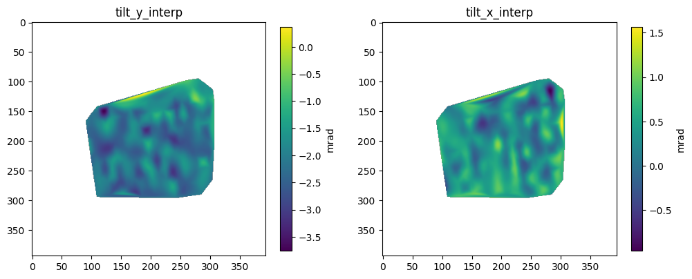
tilt_y (min, mean, max) = (-3.74, -2.08, -0.48) mrad
tilt_x (min, mean, max) = (-0.96, 0.36, 1.48) mrad
Note:#
If you want to directly plug in these values as a fixed global tilt correction, just modify your .yaml param file as:
'tilt_params' : {'tilt_type':'all', 'init_tilts':[[<TILT_Y>, <TILT_X>]]}
Replace <TILT_Y> and <TILT_X> with actual numerical values.
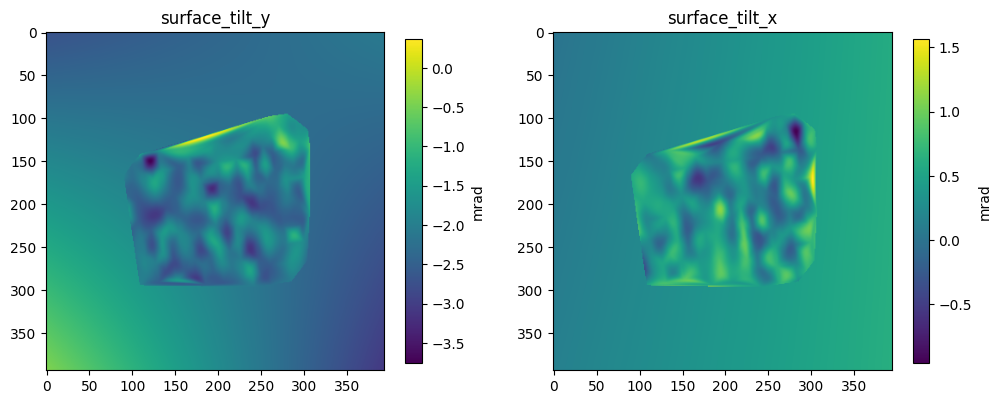
06. Fit again with simple polynomial surface to extrapolate the entire FOV#
# Use curve_fit to extrapolate to the entire FOV

def surface_fn(t, a1, b1, c1, d):
    y,x = t
    return  a1*x + b1*y + c1*x*y + d

xdata = np.vstack((Y,X))
ydata_tilt_y = tilt_y
ydata_tilt_x = tilt_x
popt_tilt_y, _ = curve_fit(surface_fn, xdata, ydata_tilt_y)
popt_tilt_x, _ = curve_fit(surface_fn, xdata, ydata_tilt_x)

# Implanting griddata interpolated values into the fitted background
surface_tilt_y = surface_fn(np.stack((ynew,xnew)), *popt_tilt_y)
surface_tilt_x = surface_fn(np.stack((ynew,xnew)), *popt_tilt_x)

mask_tilt_y = ~np.isnan(tilt_y_interp)
surface_tilt_y[mask_tilt_y] = tilt_y_interp[mask_tilt_y]
mask_tilt_x = ~np.isnan(tilt_x_interp)
surface_tilt_x[mask_tilt_x] = tilt_x_interp[mask_tilt_x]

fig, axs = plt.subplots(1,2, figsize=(12,6))
im0=axs[0].imshow(surface_tilt_y)
im1=axs[1].imshow(surface_tilt_x)
axs[0].set_title("surface_tilt_y")
axs[1].set_title("surface_tilt_x")
cbar0 = fig.colorbar(im0, shrink=0.7)
cbar0.ax.set_ylabel('mrad')
cbar1 = fig.colorbar(im1, shrink=0.7)
cbar1.ax.set_ylabel('mrad')
plt.show()
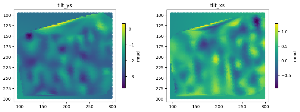
07. Sample position-dependent tilts from the extrapolated tilt field#
# Get the actual probe position on object
pos = ckpt['model_attributes']['crop_pos'] + ckpt['optimizable_tensors']['probe'].shape[-1]//2
pos
array([[ 97,  97],
       [ 97, 100],
       [ 97, 103],
       ...,
       [297, 291],
       [297, 294],
       [297, 297]], dtype=int32)
# Sample the surface with our probe position
tilt_ys = surface_tilt_y[pos[:,0], pos[:,1]]
tilt_xs = surface_tilt_x[pos[:,0], pos[:,1]]
obj_tilts = np.stack([tilt_ys, tilt_xs], axis=-1)

fig, axs = plt.subplots(1,2, figsize=(12,4))
im0=axs[0].scatter(x=pos[:,1], y=pos[:,0], c=obj_tilts[:,0])
im1=axs[1].scatter(x=pos[:,1], y=pos[:,0], c=obj_tilts[:,1])
axs[0].invert_yaxis()
axs[1].invert_yaxis()

axs[0].set_title("tilt_ys")
axs[1].set_title("tilt_xs")
cbar0 = fig.colorbar(im0, shrink=0.7)
cbar0.ax.set_ylabel('mrad')
cbar1 = fig.colorbar(im1, shrink=0.7)
cbar1.ax.set_ylabel('mrad')
plt.show()
08. Save the estimated pos-dependent obj tilt to disk#
save_array(obj_tilts, file_dir='H:/workspace/ptyrad/', file_name='obj_tilts', file_format='hdf5', append_shape=True, dataset_name='obj_tilts')
Saving array with shape = (4096, 2) and dtype = float64
Note:#
To load the estimated pos-dependent obj tilt into PtyRAD, just modify your .yaml param file as:
tilt_source : 'file'
tilt_params : {'path': '<FILE_PATH>', 'key': 'obj_tilts'}
Replace <FILE_PATH> with actual path string that points to your saved tilt file.
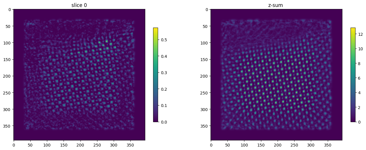
09. Reconstruct again with corrected obj tilt#
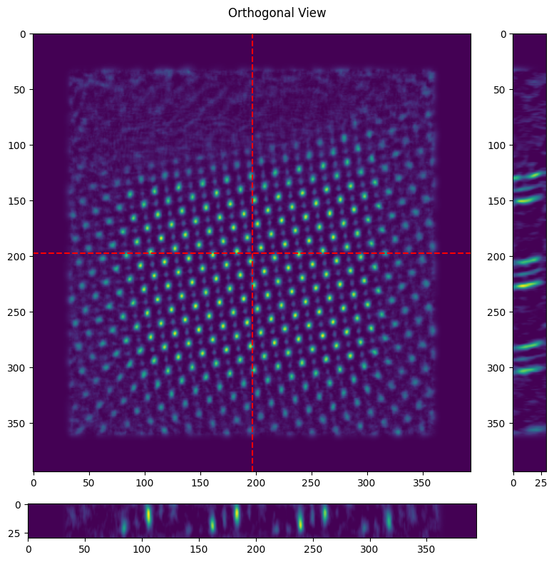
The slanted atomic column is now mostly stright, and the object z-sum is now much sharper after the tilt correction.
model_path = "H:/workspace/ptyrad_work/output/Hongbin_STO_16/20250923_full_N4096_dp128_sparse32_p4_1obj_30slice_dz10_plr1e-4_oalr5e-4_oplr5e-4_slr5e-4_dpblur1.0_orblur0.4_ozblur1.0_oathr0.95_oposc_sng1.0_spr0.1_tilt-2.4_0.27/model_iter0200.hdf5"
ckpt = load_ptyrad(model_path)
dx = ckpt['model_attributes']['dx']
slice_thickness = ckpt['optimizable_tensors']['slice_thickness']
imstack = ckpt['optimizable_tensors']['objp'].sum(0) # objp (omode, Nz, Ny, Nx) so we first reduce the omode dimension
Npix = ckpt['optimizable_tensors']['probe'].shape[-1] # Probe window size

# Plot the selected slice and z-sum
idx = 0
fig, axs = plt.subplots(1,2, figsize=(16,6))
im0 = axs[0].imshow(imstack[idx])
im1 = axs[1].imshow(imstack.sum(0))

axs[0].set_title(f"slice {idx}")
axs[1].set_title("z-sum ")

fig.colorbar(im0, shrink=0.7)
fig.colorbar(im1, shrink=0.7)
plt.show()

# Plot the orthogonal view, obj tilt is visualized by the slanted atomic column along depth dimension
ortho_view = (imstack.shape[-2]//2, imstack.shape[-1]//2) # y, x in object pixel
fig = plt.figure(figsize=(8,8))
gs = gridspec.GridSpec(2, 2, figure=fig, width_ratios=[1,0.1], height_ratios=[1,0.1])

ax0 = fig.add_subplot(gs[0, 0])
ax1 = fig.add_subplot(gs[0, 1])
ax2 = fig.add_subplot(gs[1, 0])

im0 = ax0.imshow(imstack.sum(0), aspect='equal')
im1 = ax1.imshow(imstack[:, :, ortho_view[1]].T, aspect='equal')
im2 = ax2.imshow(imstack[:, ortho_view[0], :], aspect='equal')

ax0.axhline(ortho_view[0], color='red', linestyle='--')
ax0.axvline(ortho_view[1], color='red', linestyle='--')

plt.suptitle('Orthogonal View')
plt.tight_layout()
plt.show()